
This is the second post in my three part series on the Epoch Capabilities Index (ECI). For background on the ECI and my replication of Epoch’s process of constructing it see the first post. See part three (upcoming) for multidimensional extensions of ECI, the relative importance of different benchmarks for calculating the ECI, and whether the trend in ECI improvements has been speeding up.
Introduction
In the first post of this series I replicated Epoch’s exact method for constructing the ECI. In this post I explore alternative models, and see how they impact the results and model fit. However I will first discuss the process Epoch use to construct their confidence intervals for the ECI, and why I think they might not be appropriate, and how Bayesian models could be a superior alternative.
Note that while I found some issues with the data used to construct the ECI in the first post, for this post I will continue using the same underlying data as accessed on 2026/02/04. In part three of this series (upcoming) I will look at the impacts of any updates to the data.
Uncertainty
As discussed in the last post, Epoch use (non-hierarchical) bootstrapping to produce the confidence intervals for their ECI results. The idea of bootstrapping is to repeatedly resample with replacement from the data as ways of estimating what the data ‘could have been’. This is a powerful and flexible approach, but to be valid it relies on having enough datapoints that the resamples are representative of real world data.
While ~1250 benchmark results contribute to the ECI overall, the average number of results per LLM is just 8.7 and the minimum for inclusion is only 41. This matters because the ECI model is naturally hierarchical (the data is grouped by benchmark/LLM), which makes the conditions for bootstrap validity more demanding. It’s not enough to have a large total sample; we also need sufficient data within each group, and per-LLM counts this low mean the theoretical guarantees that justify bootstrapped confidence intervals don’t apply.23
Fortunately there is an alternative, as using Bayesian statistics lets us sidestep bootstrapping entirely, and directly model the hierarchical structure. Bayesian models naturally produce uncertainty estimates as part of their fitting process, giving us valid CIs4 as long as we can come up with reasonable prior distributions for our parameters.
Loss
As covered in part 1 the original ECI model finds the parameters that minimise the following loss function:5
where
This is a frequentist approach to statistical modelling, finding the single set of parameter values that best fits the data given the specified model.
However a penalised regressions, such as the one above, can also equivalently be viewed6 as finding modal result of a corresponding Bayesian model (the ‘maximum a posteriori’ (MAP) estimator).
Considering this equivalent Bayesian model has a number of benefits. Firstly, as discussed in the previous section, Bayesian models can generate principled uncertainty estimates without relying on bootstrapping. Secondly it makes it natural to consider model extensions (like allowing different benchmarks to have different noise levels) that would be awkward to motivate as changes to a loss function but are straightforward as modelling choices. I explore this in the next section.
Bayesian Models
Base
As discussed above we can directly convert Epoch’s frequentist model into a Bayesian model with equivalent loss, obtaining the likelihood:
With priors on the parameters:
Note the sigma parameter here is not present in the original frequentist model7 but is required there to be a sensible interpretation of the model predictions when doing the goodness of fit checks covered later in this post.8
The model is otherwise kept as similar as possible to the frequentist model, with WinoGrande being used to set the scale by having its discrimination parameter fixed to 1, and the constraints that 𝛼 ∈ [0.1,10] and C, D ∈ [-10,10] still applied.
Improved Normal
Its apparent from inspecting the Base Bayesian model that it (and thus also the frequentist model) assume the amount of noise in the benchmark scores is constant across all LLMs and benchmarks, but this doesn’t seem very likely to be true. So in this model we relax the assumption by allowing the different benchmarks to have different variances, meaning that some will be expected to be noisier than others.
The base model also models the actual scores as being normally distributed, despite the fact that they can only fall into [0,1]. We can address this by truncating the normal distribution to only allow outputs between 0 and 1 (and scaling the rest of the density accordingly).9
The likelihood looks very similar, just with a different variance parameter that is now allowed to vary by benchmark:
When making this model I also took the opportunity to make various other minor changes10 that I think are natural for Bayesian modelling, such as removing the constraints on the possible parameter values and changing the priors to a more flexible setup:
And instead of setting the scale by anchoring WinoGrande to have alpha = 1 I fix the average benchmark difficulty to 0 and slope to 111 which I think is cleaner than fixing a specific benchmark:
Improved Beta
Another natural question to consider is whether the assumption of normally distributed noise/errors is correct (even after allowing for different variances for different benchmarks as above).
As an intuition for why this might not be appropriate, under the models with normal errors we penalise a predicted score of 55% when the true score is 50% just as much as a predicted score of 95% when the true score is 90%12, even though 95% might seem intuitively further away from 90% than 55% is from 50% in a sense that matters.13
One way to deal with this is to instead assume the score score follows a beta distribution with expected value equal to the predicted score, but which instead has errors that penalise mistakes more when we get close to 0 or 1.
This just involves replacing the likelihood above with:
while leaving all priors the same (with sigma_b still being allowed to vary across different benchmarks). All this does is give us a distribution where:
So as desired we have the expected value always equal to the predicted score, but also the variance (noise) is scaled to be at its maximum at a predicted score of 0.5, but decrease as it moves away from that and closer to 0 or 1.
Implementation
I wrote Stan code (specialised software for fitting Bayesian models) to implement all three of the Bayesian models discussed above, generating posterior samples that we can use for CIs for the parameters and any derived results.
All models fit well with no errors, see the appendix for more details on the fitting parameters and convergence statistics.
Results
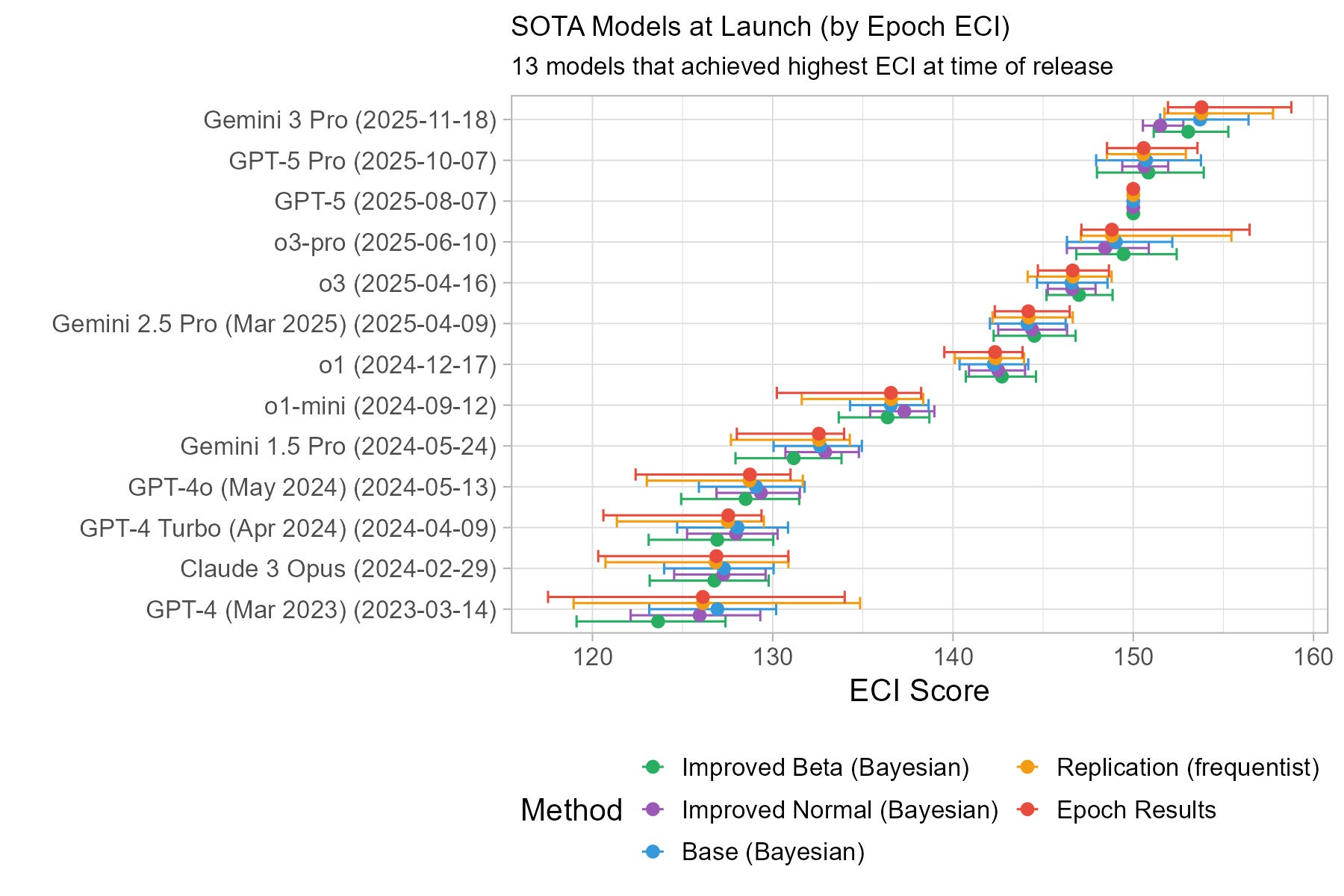
We see that the SOTA ECI results for the Bayesian models are generally very similar to the original Epoch model, but with some deviations and typically smaller confidence intervals.
We can also look in particular at which LLM the different models think is best by comparing to Gemini 3 Pro (which Epoch finds strongest currently):
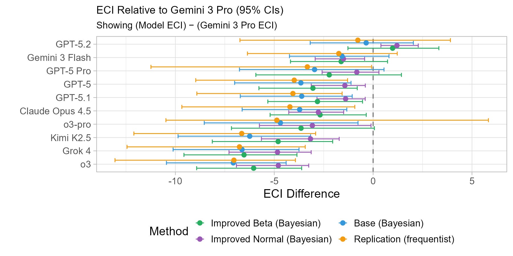
The two improved Bayesian models actually find GPT-5.2 stronger than Gemini 3 Pro, with the improved normal model finding the difference to be statistically significant at p = 0.05, but it both cases it is only a change from being 1 ECI point lower to 1 ECI point higher.
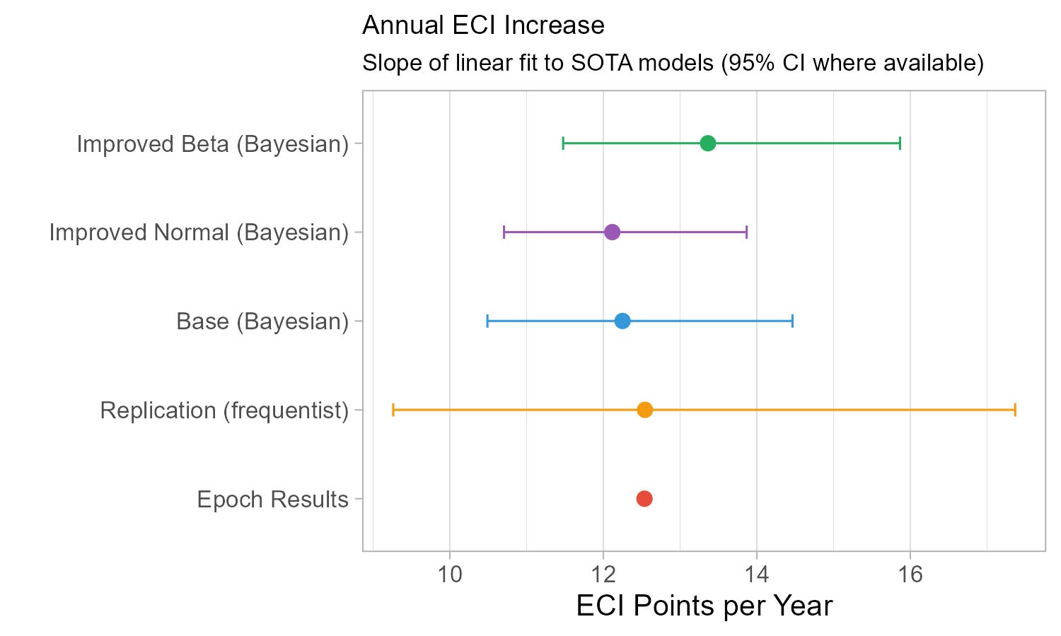
The models also have similar ECI/year trends, although the Beta model is around 10% faster than the rest (but this is within the noise of the different estimates). We will do a deeper dive into the ECI/year trends in the next post.
See full results (ECI values for every LLM and difficulty and discrimination values for every benchmark, for every model) in the appendix.
Model Comparison
We have seen the results for all the models, and I have gestured towards some theoretical considerations which might favour the Bayesian models, but it remains unclear if they should in fact be preferred. In this section we will look at various criteria on which we can compare the models, to see which fit the data best and are most predictive.
Goodness of Fit
‘Goodness of fit’ tests are one way of assessing how well a model fits the data. The general idea is picking a (hopefully quite general) feature of the data, and comparing it to how we would expect it to behave if the model is correct.
We can start with some simple examples of this, comparing QQ plots:
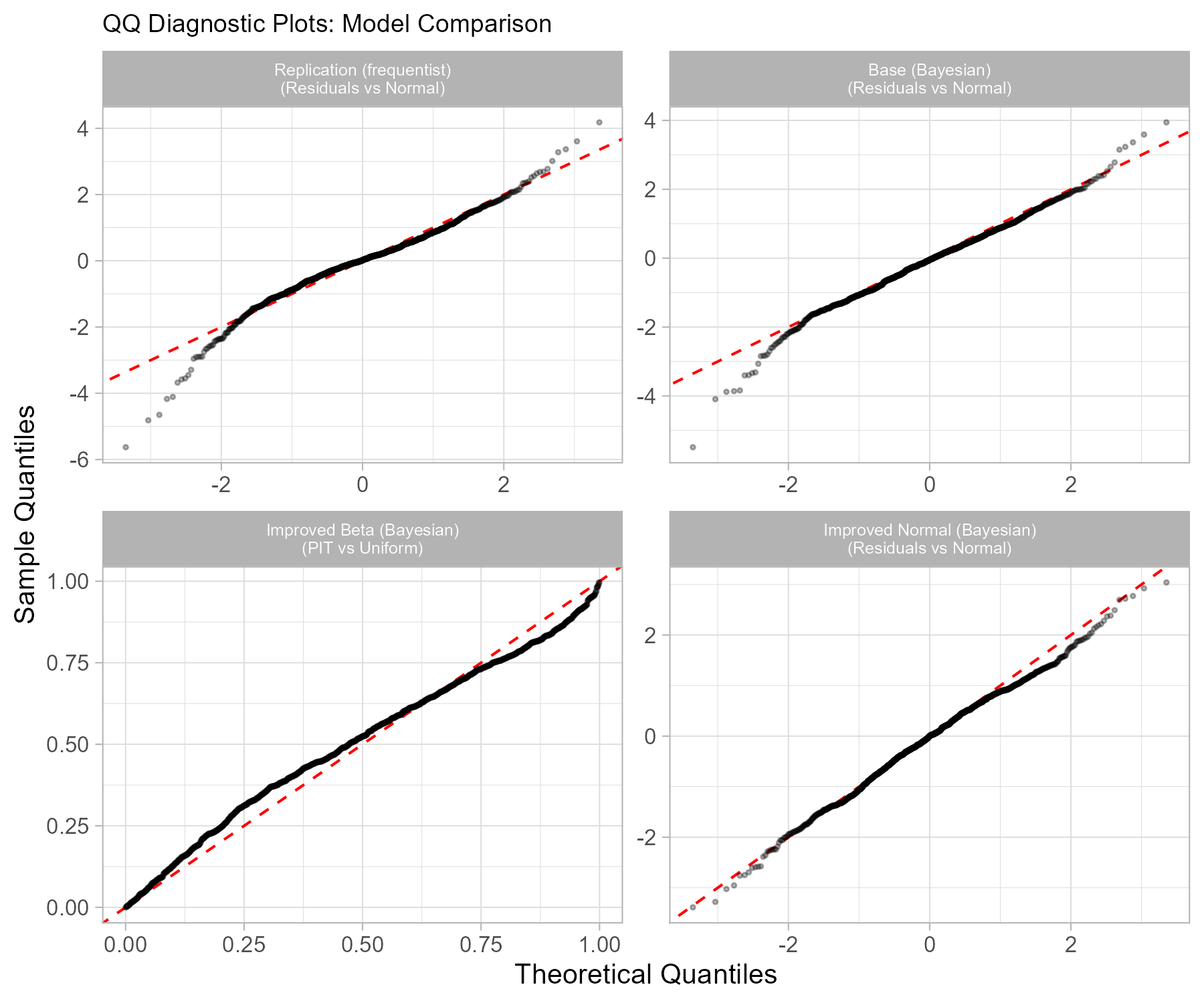
Here the frequentist model14 and the Base Bayesian model do notably worse than the improved models, with the tails coming substantially away from the main fit. Both Improved models still have some issues, with the beta having modest deviation in the mid-low and mid-high sections15, and the improved normal struggling mostly at the upper tail.
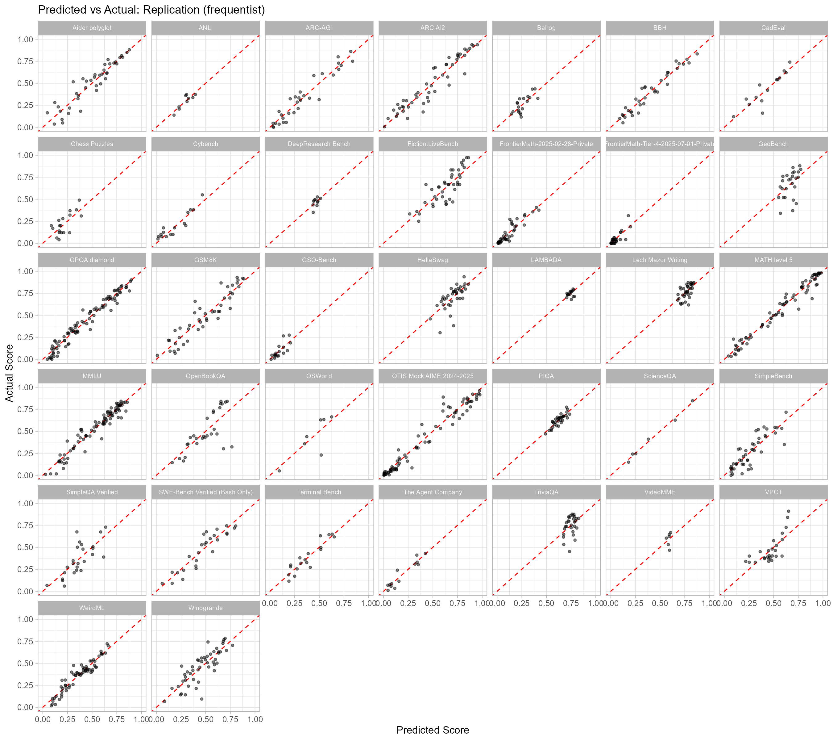
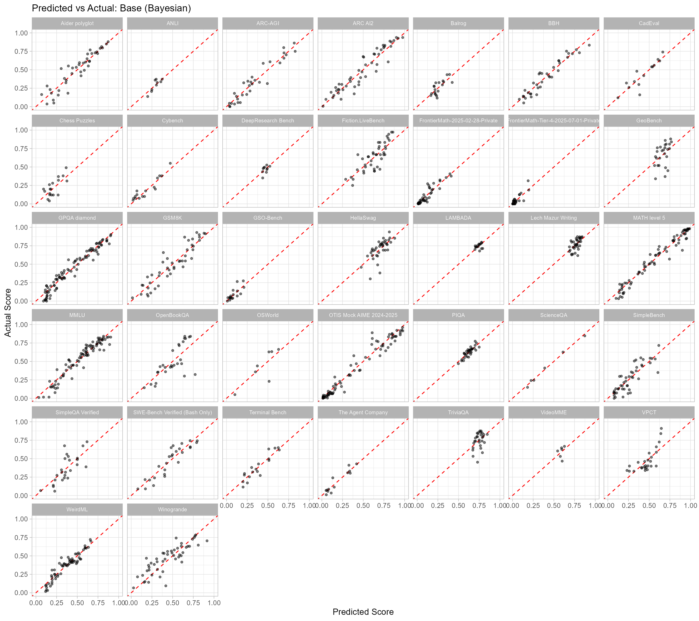
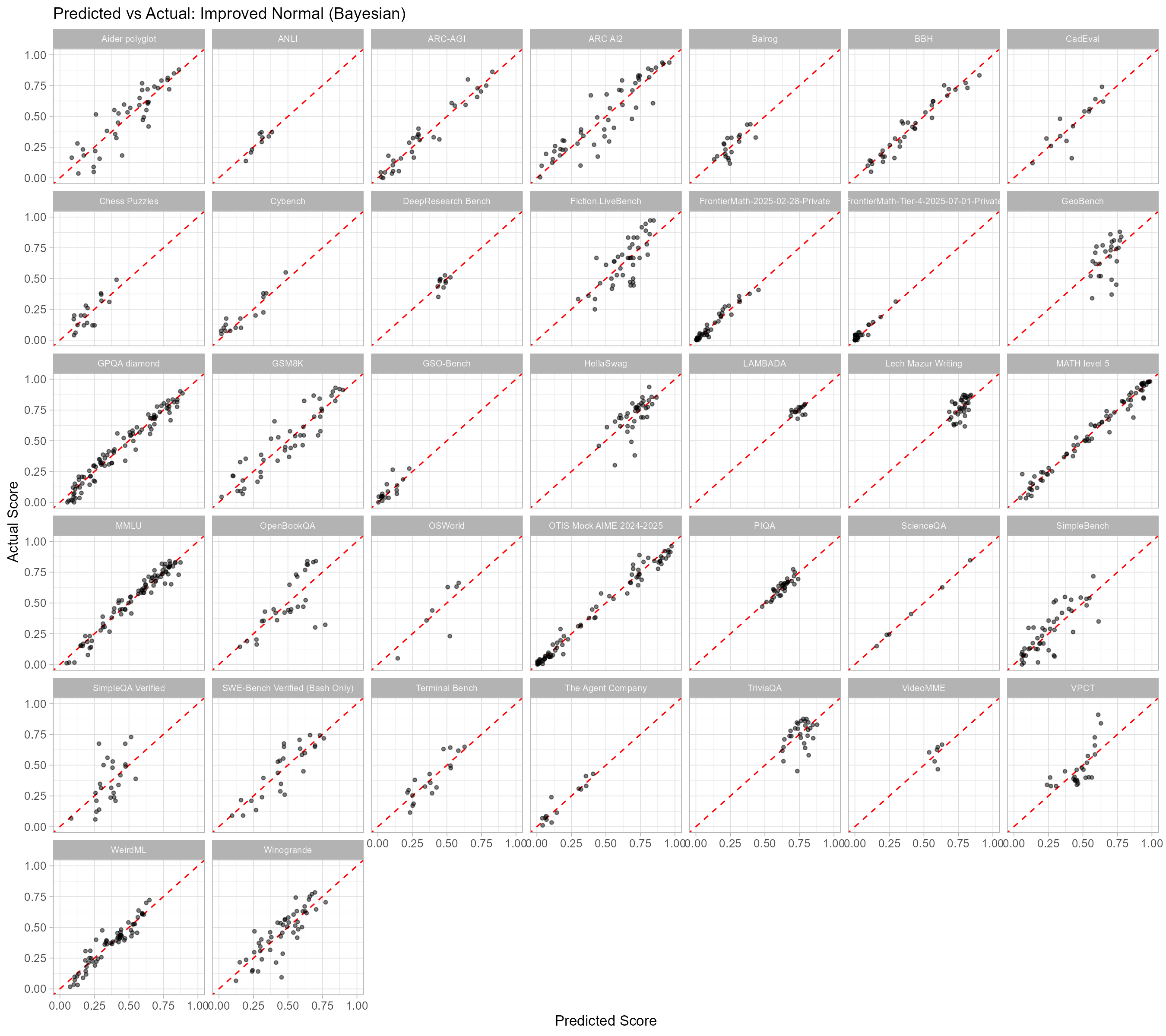
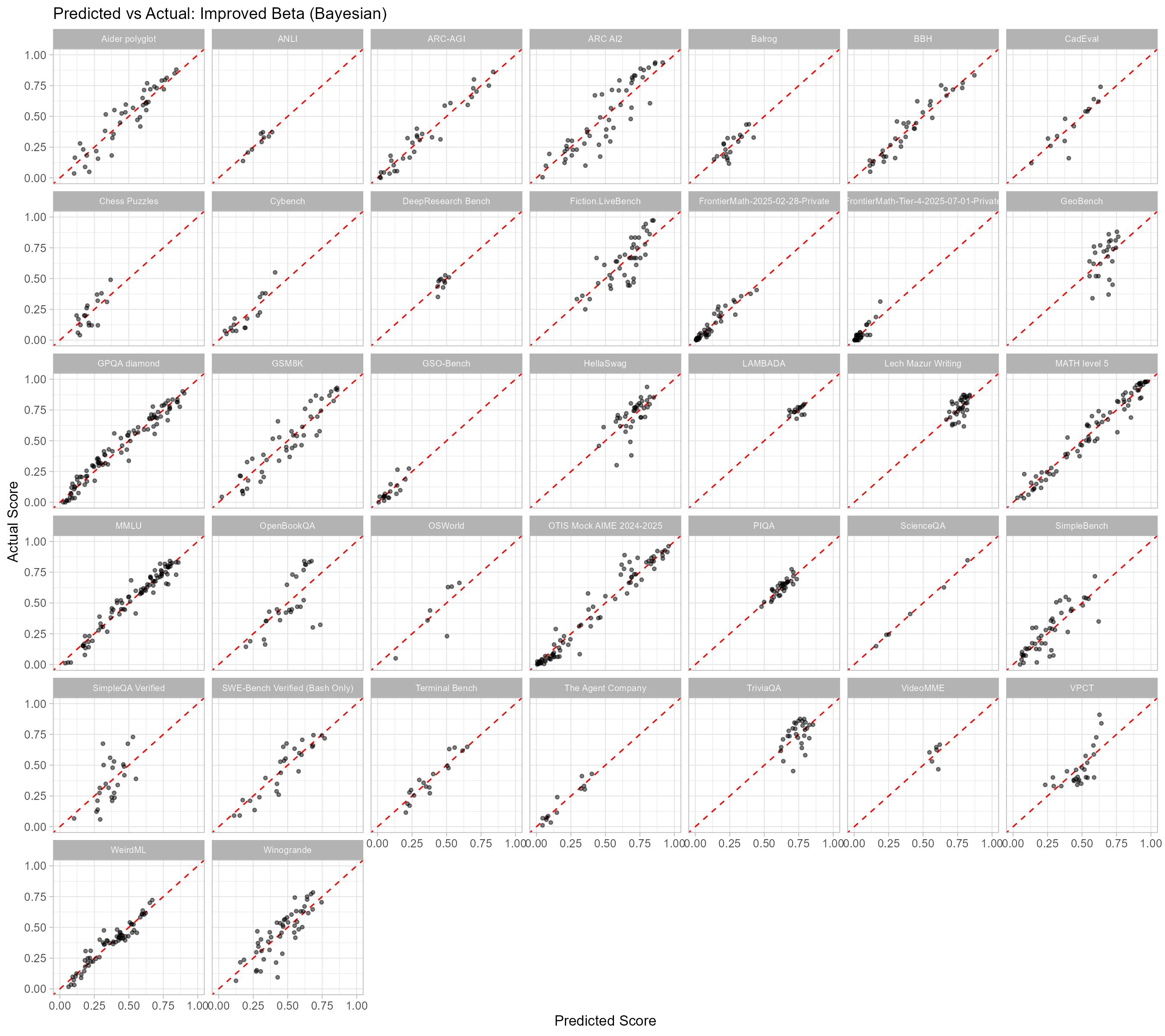
Also see the appendix for a full set of predicted vs actual plots for each model broken down by benchmark.
I also looked at the ‘Posterior Predictive P-values’ (PPP) by comparing the size of the squared Pearson residuals for the actual data to those simulated from the posterior predictive distribution of each model. Here p values correspond to the chance of the models producing data more extreme than the data we actually saw, and values close to 0.5 are ideal, with values close to 0 or 1 being concerning:
Frequentist: Method not applicable, but fit should be similar to Base Bayesian model
Base: p = 0.03 (pretty concerning)
Improved Normal: p = 0.062 (somewhat concerning)
Improved Beta: p = 0.399 (good)
We can also break these down per benchmark (where ideally each benchmark would also be close to p=0.5):
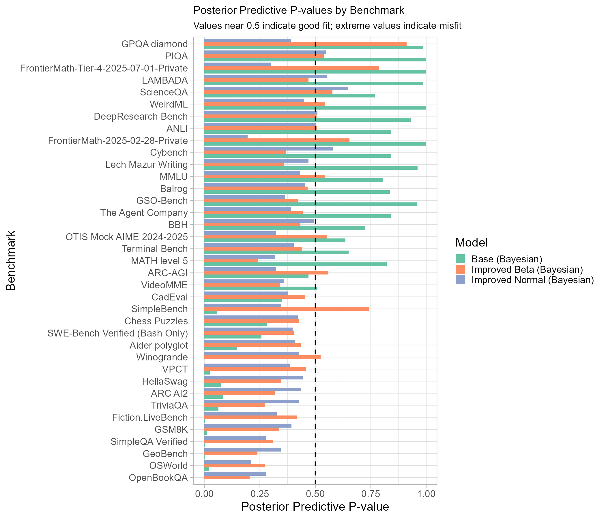
This makes it clear how poorly the assumption of constant variance across benchmarks fits the data, since for the Base model for most benchmarks it either expects more or less noise than we saw in the data (corresponding to p values close to 0 to 1). The improved models both stay much closer to 0.5 across the set of benchmarks. The Improved Normal model underpredicts noise on average, whereas the Improved Beta has a mix of under and overpredicting.
Cross Validation
An alternative approach to assess the models is to see how well they fit on new data that wasn’t included when they were being trained. Even without new data we can simulate this by using leave one out cross validation (LOO CV).16
It isn’t immediately clear what the correct measure of error to use for this is, so I look at the squared error (which Epoch’s model is trained to minimise), the mean absolute error, and a scaled version of the squared error that penalises errors more strongly when they are closer to 0 or 117:
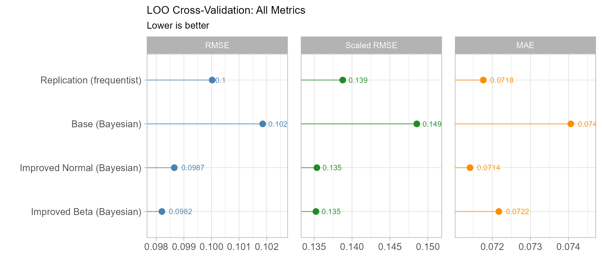
We see that the improved Bayesian models do best, each winning on one measure and both essentially drawing on the scaled RMSE, and both beating the base and replication models on most measures, although the frequentist model slightly beats the Improved Beta on MAE.
Another measure (only available for the Bayesian models) is the Expected Log Posterior Density (ELPD),18 which is less interpretable but has the advantage of allowing us to compute confidence intervals for the size of difference between models:
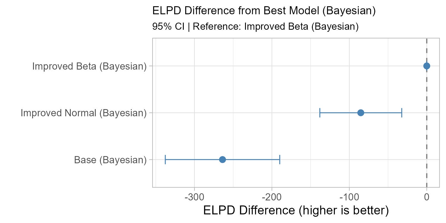
Here the Improved Beta model does best, and with the 95% CIs for the other models not overlapping zero.
Improved Beta Seems Best
Since it has by far the best posterior predictive p value, and wins on most of the cross validated error metrics I conclude the Improved Beta Bayesian model is the best fit for the data, and will use it as the basis for the analysis in post 3 (upcoming).
The Improved normal model also has a good showing however, and I suspect the ‘true’ distribution of the data is somewhere in between, with benchmark noise declining close to 0/1 but not quite in the manner the beta model assumes.19
I recommend Epoch move to this kind of model (or some further refinement) for the ECI calculations, although it is worth noting that the differences between the ECI results from the different models is usually only 1-2 ECI points (although there can be more disagreement for the very weak models, see the appendix), and there is heavy overlap of the CIs in every case.
Conclusion
Epoch’s ECI relies on bootstrapping for its confidence intervals, but the hierarchical structure and low number of benchmark results per LLM means this has unclear theoretical support. Moving to Bayesian models sidesteps this entirely, producing uncertainty estimates as a natural part of fitting the model.
I investigated three Bayesian alternatives to Epoch’s model: first directly translating Epoch’s model to a Bayesian framework, second allowing benchmarks to have different amounts of noise in their results (‘Improved Normal’) and making other minor improvements, and third assuming less noise when scores are close to 0% or 100% (the ‘Improved Beta’ model). This last model performs best overall in terms of cross-validated error and the goodness of fit checks I performed.
The resulting ECI values are generally very similar to Epoch’s, but with some differences; most notably narrower CIs and a (small) change in the top ranked LLM, with both improved models giving GPT 5.2 a higher ECI than Gemini 3 Pro. I recommend Epoch consider adopting this kind of model, although the practical differences are usually small.
In part three (upcoming) I will use the ‘Improved Beta’ model to explore further extensions of the ECI model, and also look at the relative importance of different benchmarks and whether the trend in ECI improvements has been speeding up.
Appendix
Bayesian Model Convergence
I ran each model on 4 chains, each with 4000 warmup and sampling iterations. adapt_delta was set to 0.95 and max_treedepth to 12. Each model takes around 10 minutes to fit.
All models mixed well, with no divergence transitions or max treedepth hits. The largest rhat value was 1.01, the smallest E-BFMI was 0.4 and the smallest ESS (tail and bulk) was 183, although that was only in the base model, and the other two have >400.
Replication code is available here.
Full LLM Results
Full Benchmark Results
Predicted vs Actual Scatterplots
Frequentist
Base (Bayesian)
Improved Normal (Bayesian)
Improved Beta (Bayesian)
The smallest benchmark has 10 results, with an average of 33.7.
We also need there to be large numbers enough of benchmarks and LLMs themselves, although this is likely satisfied with the 37 benchmarks and ~150 LLMs.
As discussed in the first post Epoch actually use a non-hierarchical bootstrap setup - but I think this is doubly inappropriate; I think a hierarchical bootstrap would both be more valid (due to the hierarchical structure of the data) but still not well theoretically justified (because of the low number of data points per LLM).
Technically Bayesian Models produce Credible Intervals as opposed to frequentist Confidence Intervals. While extremely long debates are possible about the merits and interpretations of both, for the purposes of these posts I will use and describe both interchangeably as ‘CIs’.
For more details see the first post.
Since it just controls the overall scale of the loss, but this means it isn’t required for finding the parameter values that minimise it in the original penalised regression.
I gave it a uniform prior to minimise the amount that it would contribute to the loss when fitting the model, to keep things as close to the frequentist model as possible.
This means that the true mean and variance of the distribution do not match the distributions parameters, but since it mostly seems like the model should be able to learn around this I took no steps to address it, and leave it as an extension for further work. When calculating the Pearson residuals I use the true mean and variance of the truncated distribution.
Ideally I would consider the impact of each change in isolation, but as I believe these adjustments are individually well-motivated and for the interest of time I will just combine them.
On the untransformed scale before we convert Claude Sonnet 3.5 to 130 and ChatGPT 5.0 to 150.
Since in any model with normally distributed errors (or in Epoch’s model) the loss is a function of just (predicted - actual), which is 0.05 in both cases.
One way to think about this would be considering the relative error instead of the absolute error.
To standardise the residuals for the frequentist model I used their observed standard deviation.
The beta QQ plot here uses an alternative method (PIT vs uniform) to the direct quantile comparisons in the other two plots, so its shape isn’t directly comparable, but it remains the case that a perfect fit would be a straight line on y=x.
For the replication model I compute the LOO CV directly, but as the Bayesian models take longer to fit I instead use the PSIS-LOO approximation from the loo R package. On each Bayesian model ~50/1248 samples have high pareto-k values which indicate they might have biased results, but in the interests of time I did not investigate or address this.
This is constructed by scaling each residual by min(10, 2/sqrt(p(1-p))) where p is the actual value observed.
Also calculated using PSIS LOO via the loo package.
One could explore models to try and capture this behaviour, but for the interests of time I do not do this here.